Professor: Steve Marschner · TAs: Mariia Soroka and Gemmechu Hassena
Final Image
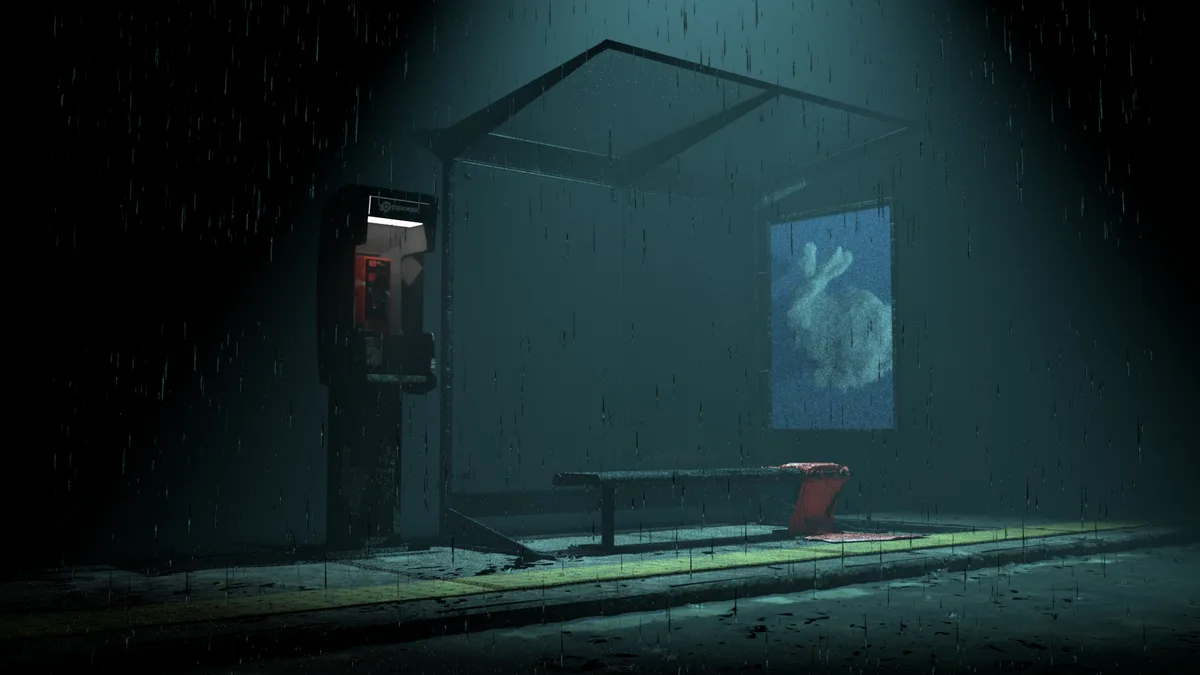
On a quiet rainy night, an empty bus station is wrapped in cold blue light and drifting mist. Rain falls across the glass, pavement, and curb, turning the air itself into a visible layer of atmosphere. On the left, a red phone booth glows like the only warm object in the scene, standing alone against the darkness.
A piece of red silk cloth rests on the bench, soft and saturated against the otherwise cold environment, as if someone had just left it behind. The advertisement panel shows a rabbit with a slightly flickering screen-like texture, adding an unstable, dreamlike detail to the station. The scene is meant to feel like a brief pause in the city: no character is visible, but traces of human presence remain in the objects, light, rain, and silence.
Texture Mapping
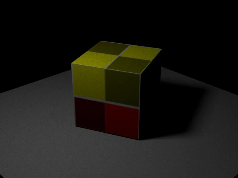
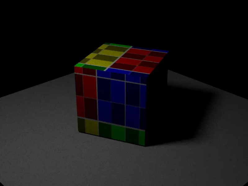
This feature lets Nori read image textures from mesh UV coordinates and use them as material inputs. The implementation is used both by small texture test scenes and by imported Blender scenes such as the bus station assets. Texture lookup uses bilinear interpolation between neighboring texels, which makes magnified texture samples smoother than nearest-neighbor lookup.
Qualitative validation
Quantitative validation against PBRT
I built a matching PBRT v4 scene with the same camera, cube UVs, checker texture, diffuse material, floor, and area
light. PBRT uses simplepath with maxdepth=1, direct light sampling enabled, and BSDF path
continuation disabled, matching the direct-lighting setup used by the Nori scene. Both renders use 64 spp. The PBRT reference image is
horizontally flipped to match Nori's image-space orientation, and the checker texture is vertically flipped for PBRT
so that both renderers sample the same UV image orientation. The image grid uses PNG previews, while the global MSE and
per-pixel error image are computed directly from the corresponding linear EXR pixels at 800x600 resolution.
I suspect that part of the remaining difference comes from PBRT's spectral rendering pipeline, while my Nori
implementation only supports RGB-valued rendering.
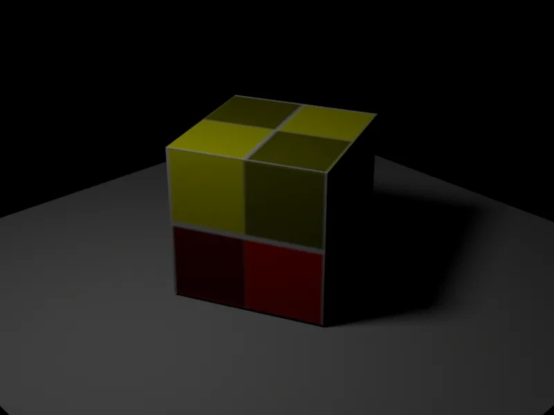

[0, 1] actual MSE scale.
[0, 1e-2] scale.
Source EXRs:
texture_mapping.exr and
texture_mapping_pbrt.exr.
| Metric | Value |
|---|---|
| Global MSE | 1.11557147e-05 |
- The preview images are tonemapped PNGs, while the MSE is computed from linear EXR data.
- The per-pixel MSE is computed as mean squared RGB error for each pixel, then averaged over the full image for the global value.
- Most remaining error comes from renderer differences in texture filtering, area-light sampling, and color handling.
- The first heatmap uses a
[0, 1]actual MSE range so near-zero differences remain black; the second uses[0, 1e-2]to reveal small residual structure.
Normal Mapping
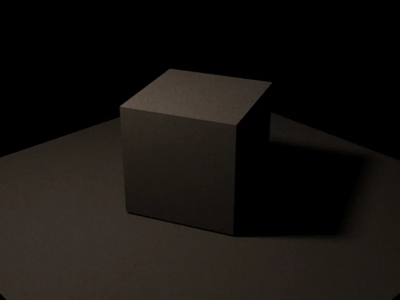
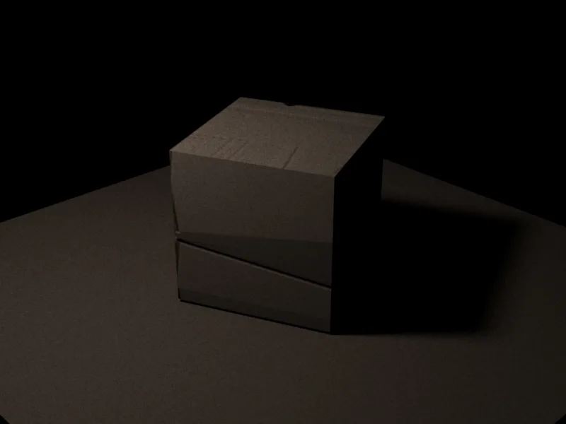
Normal mapping adds visual surface detail without changing the actual mesh geometry. The cube is still made of flat faces, but each point on the surface reads a normal direction from the normal map texture and uses that direction for shading. This changes how light reflects across the surface, making the flat face look bumpy or detailed while the silhouette remains unchanged. In my implementation, the RGB normal map is decoded as a tangent-space normal, transformed into world space using the mesh UV derivatives, and then used by the diffuse or Disney BRDF when evaluating lighting.
Qualitative validation
Quantitative validation against PBRT
I built a matching PBRT v4 scene with the same camera, cube UVs, normal map texture, gray diffuse material, and area
light. PBRT uses simplepath with maxdepth=1, direct light sampling enabled, and BSDF path
continuation disabled, matching the direct-lighting setup used by the Nori scene. Both renders use 64 spp. The PBRT reference image is
horizontally flipped to match Nori's image-space orientation. The image grid uses PNG previews, while the global MSE and
per-pixel error image are computed from the corresponding linear EXR pixels at 800x600 resolution.
I suspect that part of the remaining difference comes from PBRT's spectral rendering pipeline, while my Nori
implementation only supports RGB-valued rendering.
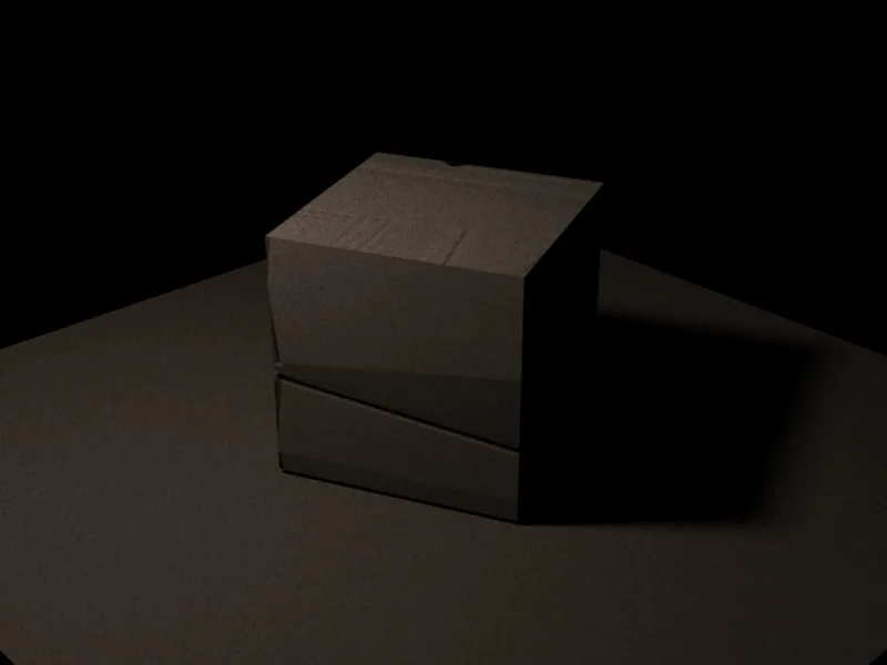
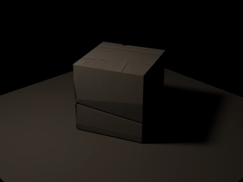

[0, 1] actual MSE scale.
[0, 1e-2] scale.
Source EXRs:
normal_mapping_gray_on_nori.exr and
normal_mapping_pbrt_gray_on.exr.
| Metric | Value |
|---|---|
| Global MSE | 4.02589194e-06 |
- The preview images are tonemapped PNGs, while the reported MSE values are computed directly from the linear EXR data.
- The PBRT reference is cleaner because PBRT's sphere area light sampling has lower variance than Nori's mesh area light sampling at the same 64 spp.
- The MSE is computed directly from the linear EXR files as per-pixel mean squared RGB error, then averaged over the full image for the global value.
- The first heatmap uses a
[0, 1]actual MSE range so near-zero differences remain black; the second uses[0, 1e-2]to reveal small residual structure.
Quantitative validation against Mitsuba
I also built a matching Mitsuba 3 scene using the same camera, cube OBJ, UV layout, normal map texture, gray diffuse
material, floor, area light, 800x600 resolution, and 64 spp. The final report image uses the V-flipped normal-map
texture convention that best matches Nori. Mitsuba's normal-map bitmap lookup uses a different
vertical UV/image convention than my Nori image texture, so the Mitsuba texture includes a to_uv
transform that flips V before sampling. After that adjustment, the normal-map features align with the Nori render.
The image grid uses PNG previews, while the global MSE and per-pixel error image are computed directly from the
corresponding linear EXR pixels.
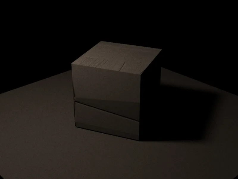

[0, 1] actual MSE scale.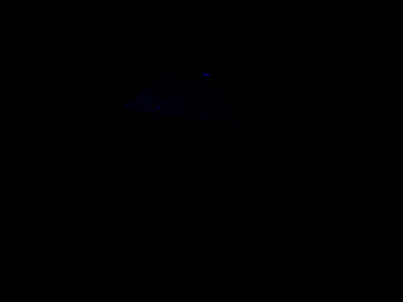
[0, 1e-2] scale.
Source EXRs:
normal_mapping_gray_on_nori.exr and
normal_mapping_mitsuba_gray_on.exr.
| Metric | Value |
|---|---|
| Global MSE | 6.74640160e-06 |
- The MSE is computed directly from the linear EXR files as per-pixel mean squared RGB error, then averaged over the full image.
- The Mitsuba scene uses the
cuda_ad_rgbvariant and RGB film output, so this comparison avoids PBRT's spectral conversion path. - Remaining differences mainly come from renderer implementation details such as image filtering, normal-map frame construction, direct-light sampling, and tonemapped PNG preview differences.
- The first heatmap uses the same
[0, 1]actual MSE range as the PBRT normal-map comparison; the second uses[0, 1e-2]to reveal small residual structure.
Heterogeneous Medium, NanoVDB, and Environment Light
The medium system supports spatially varying density, including procedural grid volumes and NanoVDB density fields.
This is used to render fog, clouds, and visible light shafts. For the cloud bunny scene, the renderer reads a
.nvdb density grid and lights it with a floating-point RGB HDR environment map. Here, HDR means that
the environment image stores high-dynamic-range RGB radiance values, not that the renderer performs spectral light
transport.
Qualitative validation
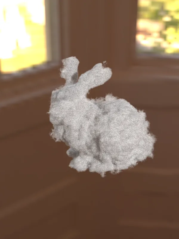
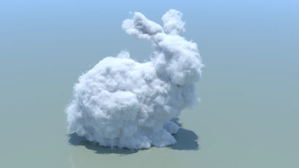
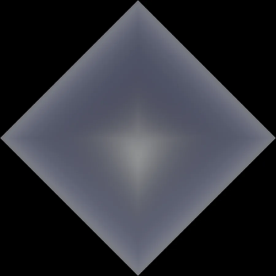
cloud_bunny_sky.exr.
Quantitative validation against PBRT
I built a matching PBRT v4 volume path tracing scene with the same camera, NanoVDB density grid, environment map, medium coefficients, HG phase parameter, and 64 spp. For the quantitative test, both renderers use the NanoVDB file's native grid/world coordinates so the comparison isolates density lookup and heterogeneous volume integration rather than an extra renderer-specific volume transform. The scene is lit only by the environment map, with no helper area light or floor, to avoid renderer-specific area-light and shadow differences. Nori evaluates the sky image as a latitude-longitude map, while PBRT v4's environment light uses a different environment-map parameterization. The PBRT image is horizontally flipped to match Nori's image-space orientation.
This comparison scene is intentionally simpler than the downloaded PBRT bunny-cloud.pbrt package scene.
The original package includes a coated diffuse ground disk, a 4x scaled and rotated HDR sky, PBRT-specific NanoVDB
rotations, a Halton sampler, camera film settings such as sensor/white balance/ISO, a 1920x1080 film, max depth 50,
and wavelength-style medium coefficients. For the quantitative Nori/PBRT comparison, I removed the ground plane and
extra light/volume rotations, matched the camera, resolution, sampler, path depth, and RGB medium parameters, and
kept only the cloud volume plus environment lighting.
This avoids comparing renderer-specific scene conventions and makes the reported MSE focus on the heterogeneous
medium and environment-light transport.
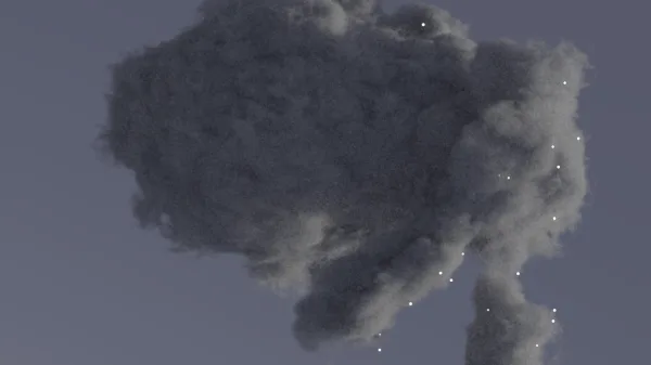
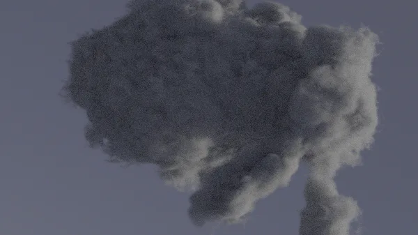
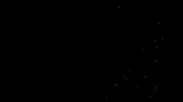
[0, 1] actual MSE scale.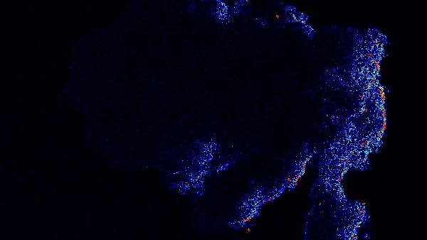
[0, 1e-2] scale.
Source EXRs:
Nori and
PBRT.
| Metric | Value |
|---|---|
| Global MSE | 1.93040874e-02 |
| Median per-pixel MSE | 7.47329905e-05 |
| 90th percentile per-pixel MSE | 6.01561682e-04 |
| 99th percentile per-pixel MSE | 4.89051314e-03 |
- The preview images are tonemapped PNGs, while the reported errors are computed directly from the corresponding linear EXR pixels at 600x337 resolution.
- The per-pixel error is the mean squared RGB difference for each pixel; the global MSE is the average of those per-pixel values over the whole image.
- The HDR environment map contains localized bright regions. With only 64 spp, a small number of medium scattering samples can hit those bright directions and create high-energy firefly pixels in the Nori render.
- Nori samples and evaluates the environment light as a latitude-longitude map, while PBRT v4's environment light uses a different sphere-map parameterization. The different parameterizations and finite sample count can still leave small sampling differences around bright envmap regions.
- Some residual error can also come from spectral-to-RGB conversion differences in the environment light and medium parameters, since PBRT's original scene uses spectrum-valued inputs while this Nori comparison uses RGB coefficients.
- My Nori implementation does not support spectral rendering and evaluates transport directly in RGB, so color or brightness differences from PBRT's spectral pipeline are most visible in bright regions where MSE strongly amplifies the residual error.
- Most pixels match closely, as shown by the low median, 90th percentile, and 99th percentile per-pixel MSE values. The higher global MSE is dominated by a very small number of unusually bright outlier pixels because MSE squares those large errors.
- The first heatmap uses a fixed
[0, 1]actual MSE scale, while the second uses[0, 1e-2]to reveal lower-magnitude spatial error around the high-variance regions.
Equiangular MIS / Volumetric Noise Reduction
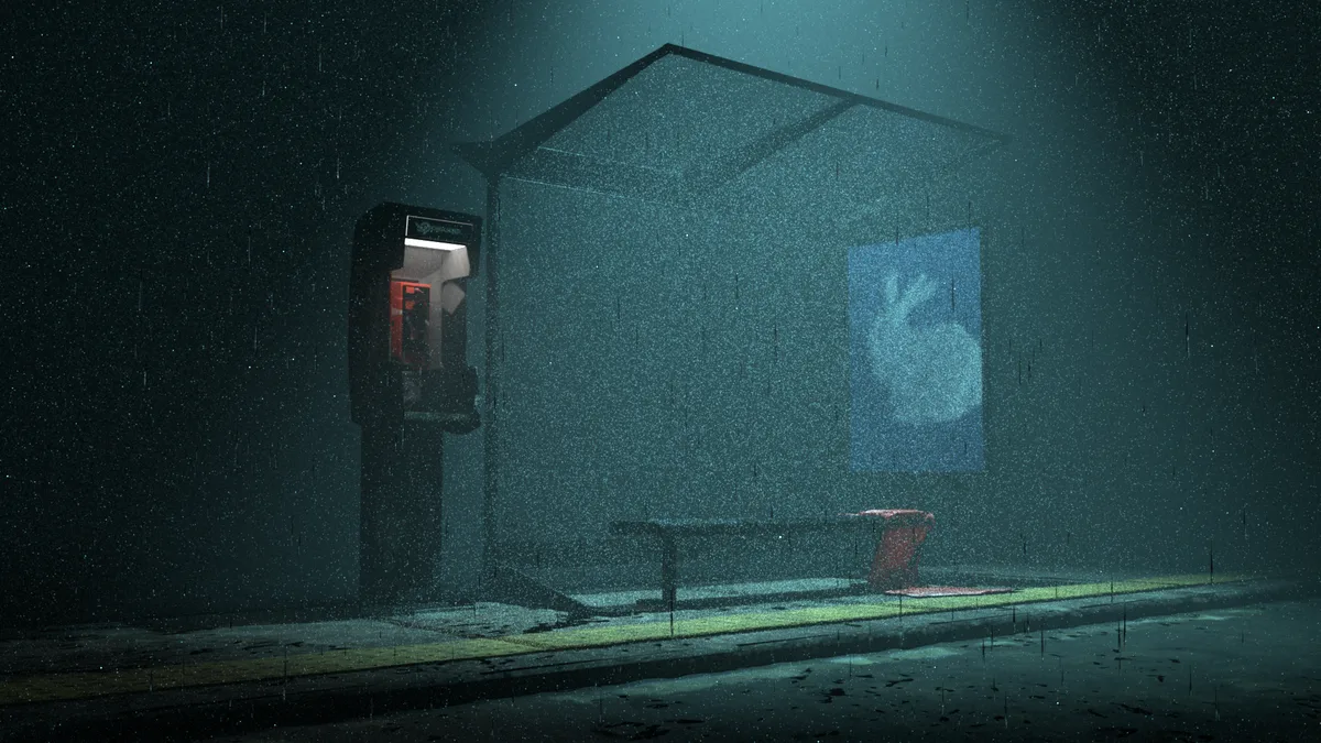
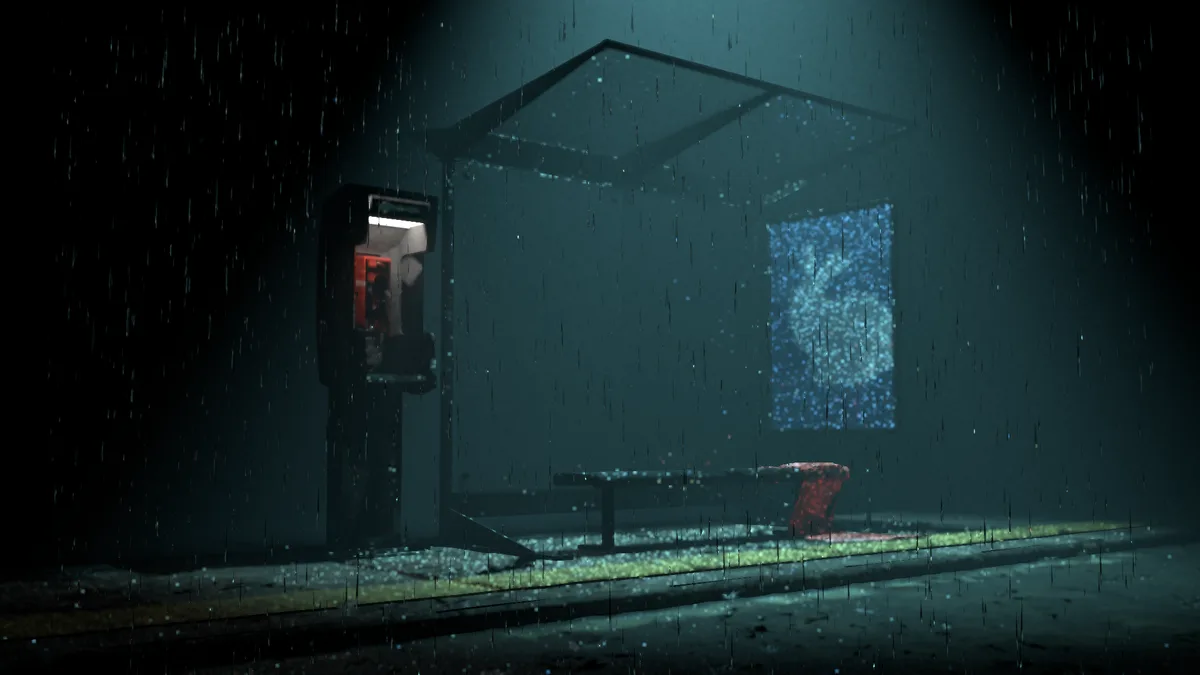
For narrow lights in participating media, the regular heterogeneous-medium random walk can spend many samples on medium events that contribute little to the visible beam. The volumetric path tracer includes an experimental equiangular MIS distance strategy to place more samples near important light paths.
The regular volumetric path tracer samples actual medium events: it samples a distance inside the medium, classifies the event as absorption, real scattering, or null collision, and for a real scattering event it samples the phase function to continue the path in a new direction. This supports multiple scattering, but a small or narrow light can still be very noisy because many sampled medium points do not contribute much to the visible beam.
My equiangular branch is a specialized single-scattering direct-lighting estimator. Instead of creating a new continuing medium vertex, it samples a point along the current camera/path ray and directly connects that point to a compact light source. The phase function is still evaluated from the light direction to the view direction, but no new phase direction is sampled in this branch, so the main ray continues forward with medium transmittance.
Compared with a no-medium path tracer, the ray geometry is similar because the main ray still reaches the same surface or environment direction. The difference is that the medium attenuates the ray by transmittance and adds in-scattered light along the way. Compared with the regular volumetric path tracer, this method is less general, but it is effective for visible shafts from compact lights because it mixes exponential distance sampling with equiangular sampling around the light position.
Thin Lens Camera
The perspective camera was extended with a thin lens model. A nonzero lensRadius samples a point on
the lens disk, while focalDistance controls which depth remains sharp.
In the final rainy bus station scene, this is also used to defocus nearby raindrops so foreground droplets do not
appear as overly sharp, distracting bright highlights.
Qualitative validation
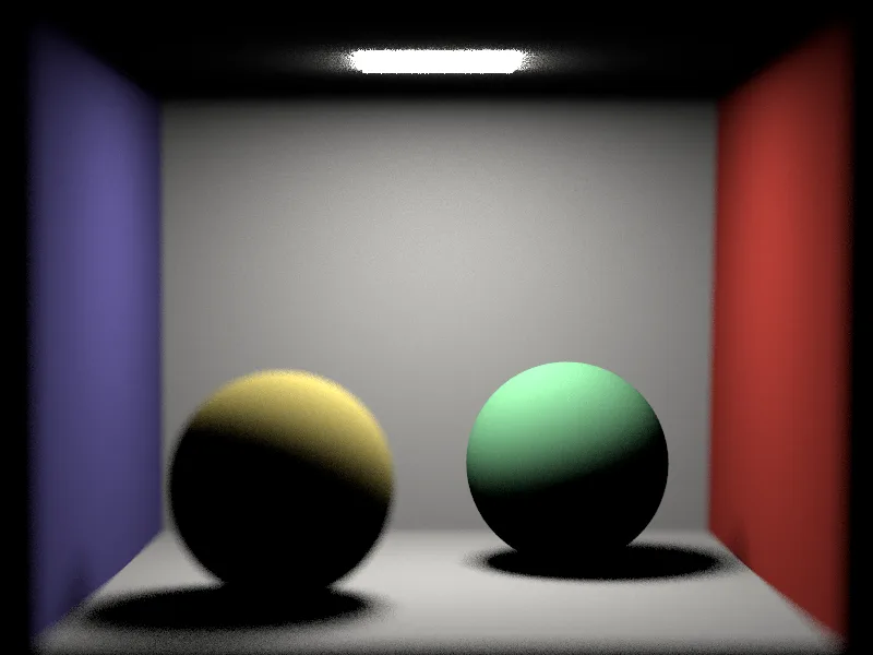
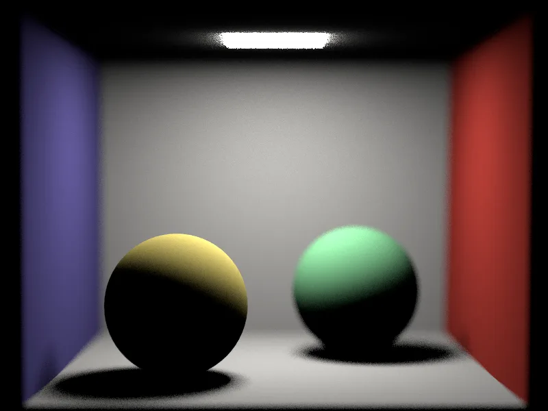
lensRadius=0.15 and 64 spp.
Quantitative validation against PBRT
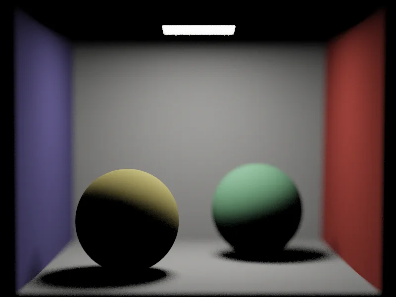
I built a matching PBRT v4 scene using the same Cornell box geometry, diffuse materials, area light, camera
transform, resolution, 64 spp, lensradius=0.15, and focaldistance=5.05. PBRT uses its
standard perspective camera with thin lens parameters, not the more complex realistic camera model, so
the comparison isolates the thin lens camera behavior. The PBRT reference is compared against the Nori near-focus
render, and the per-pixel error is computed from the corresponding linear EXR pixels at 800x600 resolution.
The colors in the PBRT and Nori previews are not perfectly identical, which may partly come from PBRT's
wavelength-sampled spectral pipeline: PBRT reconstructs spectra from RGB inputs before converting the result back to
RGB, while my Nori implementation transports RGB values directly.

[0, 1] actual MSE scale.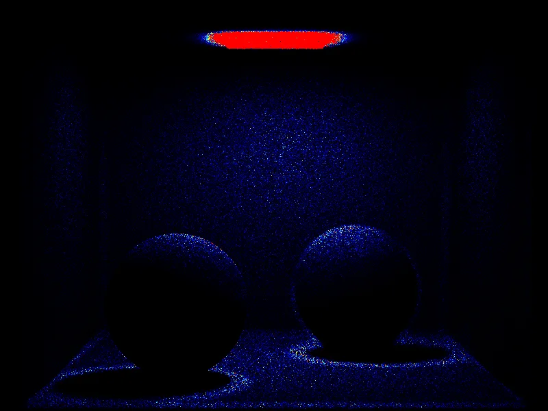
[0, 1e-2] scale.
Source EXRs:
Nori and
PBRT.
PBRT v4 accepts RGB scene inputs and writes an RGB film, but its light transport is still wavelength-sampled spectral rendering. This can leave small color and brightness differences compared with Nori's direct RGB pipeline, even when both scenes use the same RGB material and light values.
| Metric | Value |
|---|---|
| Global MSE | 5.18575728e-01 |
| Median per-pixel MSE | 3.37672027e-05 |
| 90th percentile per-pixel MSE | 5.58765780e-04 |
| 99th percentile per-pixel MSE | 5.95019106e-03 |
- The comparison grid shows tonemapped PNG previews, while the MSE values are computed directly from the linear EXR images.
- The PBRT perspective-camera reference was used without horizontal flipping for this scene; that orientation had the lowest EXR-space MSE.
- Most pixels match closely, as shown by the median, 90th percentile, and 99th percentile errors. The higher global MSE is dominated by a small number of bright outlier pixels, mainly around light-source and bright-highlight regions where small residual differences are strongly amplified by squared error.
- The first heatmap uses a fixed
[0, 1]actual MSE scale, while the second uses[0, 1e-2]to reveal lower-magnitude spatial error around the high-variance regions.
Procedural Generated Meshes: Rain Droplets and Splashes
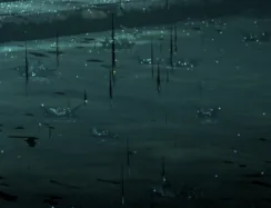
The final scene uses generated geometry for rain streaks, droplets, and ground splashes. This turns the static bus station environment into a rainy night scene and also provides animated frames for the final GIF.
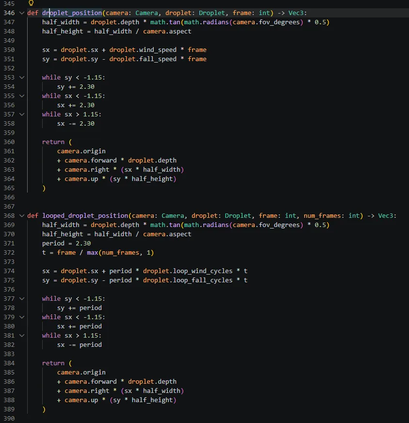
The rain is generated by scenes/final-feature-tests/busstation/generate_rain_sequence.py. The script
first builds a stable list of droplets in make_droplets(): each droplet stores a random screen-space
position, depth, scale, stretch, rotation, fall speed, and wind speed. For each frame,
droplet_position() converts the droplet from camera-space coordinates into world space using the camera
forward, right, and up vectors. The position is updated by fall speed and wind speed, then wrapped back into the
screen region so the rain density stays stable across the animation.
The mesh output is written per frame in write_merged_obj(). Each rain drop copies the same droplet
prototype OBJ, recenters it, applies its random scale/stretch/rotation, and appends it into one combined rain OBJ.
Ground splashes are more procedural: make_splashes() places them near the road and sidewalk, while
append_splash_geometry() writes a small crown-shaped mesh with randomized radius, height, phase, and
spoke count. Finally write_xml() injects the generated OBJ back into the bus station scene with a
rough dielectric water material.
Cloth / Microcylinder BSDF and Physics Simulation
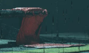
The cloth material follows Sadeghi et al.'s microcylinder appearance model. It evaluates two yarn systems, combines surface reflection and volume scattering for each thread, then applies self-shadowing and projected-length normalization.
The original curved cloth sample mesh and reference images in this section are adapted from MatchaChoco010/path_tracer_cloth, an MIT-licensed Rust implementation of the same microcylinder cloth model.
Paper-Style Table II Validation
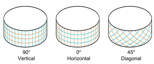
To validate the BSDF against the paper setup, I rendered two silk Table II material presets on three identical vertical
cylinders with different tangent orientations from left to right: 90 degree vertical, 0 degree horizontal, and
diagonal 45 degrees. Each panel uses 64 spp, a black background, and a large camera-side area light
(z=16, radiance=(22,22,22)) so that the RGB profiles mainly show the effect of cloth
orientation and material parameters rather than a hard point-light pattern. The RGB line plot above each render is
computed from the displayed PNG by averaging each cylinder crop vertically per image column.
Since the paper does not specify the exact cylinder dimensions or light placement for these validation plots, I had to approximate the geometry and lighting setup. This means the overall lobe locations and color trends are the main comparison target, while the exact thickness of individual bands can change if the cylinder radius, camera framing, or light size and position are adjusted.
The RGB profile curves provide the main evidence for this comparison: their peaks, valleys, and left-to-right color ordering follow the same overall distribution as the reference plots. This indicates that the cloth scattering lobes are arranged correctly for the three tangent orientations, even though the precise band widths are affected by the approximated cylinder and lighting setup.
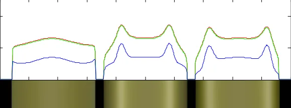
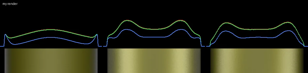
cloth_paper_silk_crepe_de_chine.png, cloth_paper_silk_crepe_de_chine.exr.
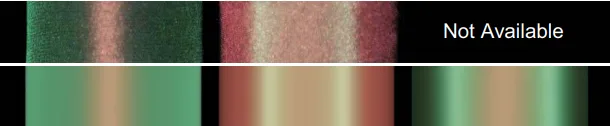
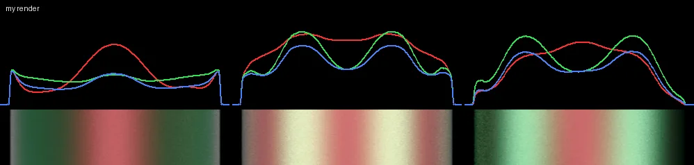
cloth_paper_silk_shot.png, cloth_paper_silk_shot.exr.
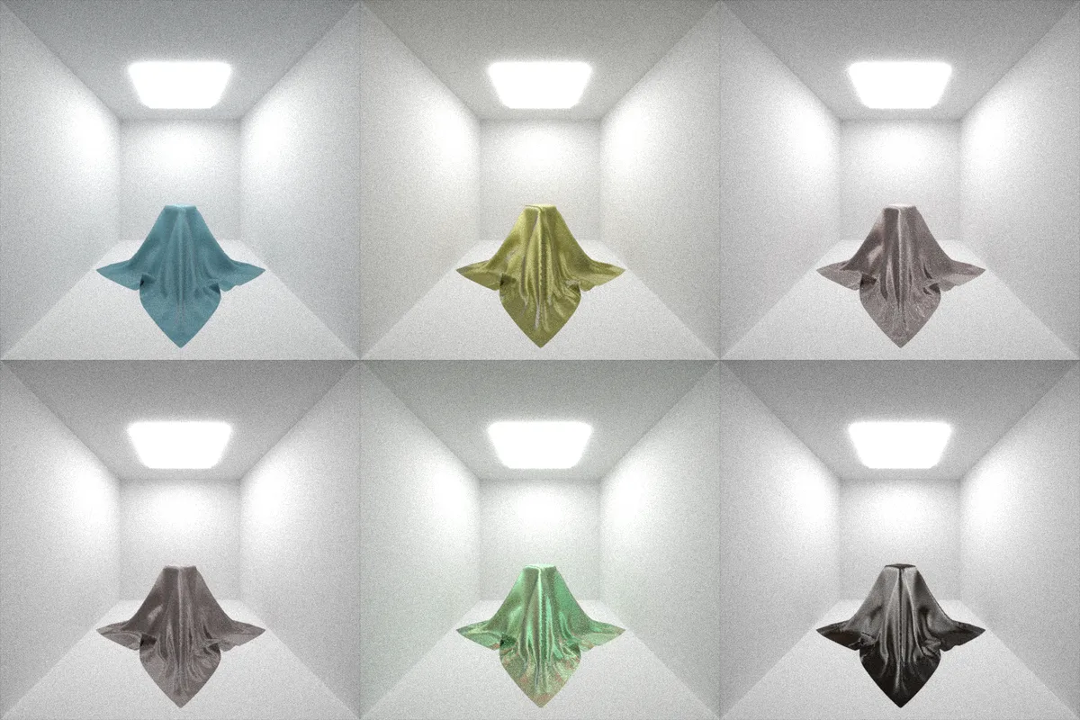
path_tracer_cloth
repository for the microcylinder material.
The following three images are my own Nori renders of the microcylinder BSDF with different color parameters.
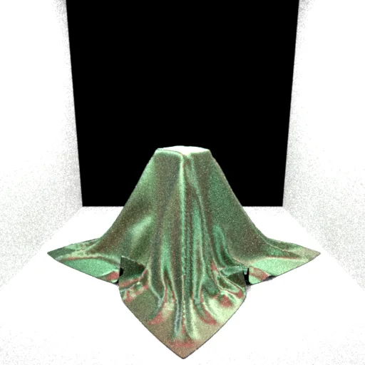
A0=(0.02, 0.20, 0.08), A1=(0.60, 0.00, 0.06).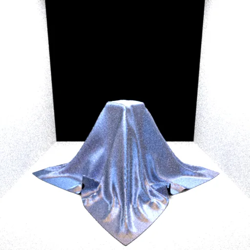
A0=(0.035, 0.145, 0.420), A1=(0.780, 0.430, 0.070).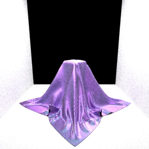
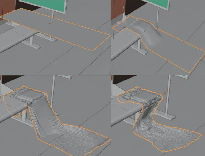
A0=(0.270, 0.060, 0.430), A1=(0.020, 0.420, 0.360).The cloth mesh itself was created in Blender using a cloth physics simulation. I used the simulation to drape and deform a subdivided surface, then exported the resulting mesh for rendering in Nori.
Stratified Sampling
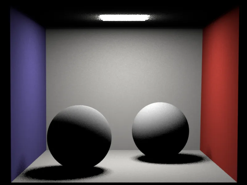
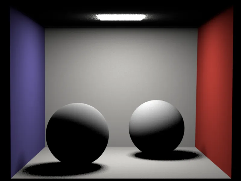
The stratified sampler divides the pixel sample domain into strata and samples each region more evenly than purely independent random sampling. This reduces visible noise patterns at the same sample count.
Disney BRDF
The Disney BRDF implementation provides a practical artist-friendly material with diffuse, metallic, roughness, sheen, clearcoat, and anisotropic controls. The final bus station scene uses it for many imported materials.
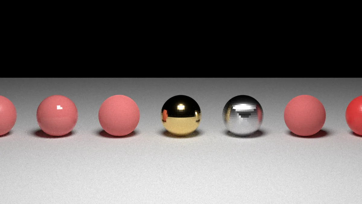
roughness=0.4), low roughness glossy plastic (roughness=0.05),
high roughness matte plastic (roughness=0.9), metallic gold
(metallic=1.0, roughness=0.12), anisotropic brushed metal
(anisotropic=0.85), cloth-like sheen (sheen=0.7,
sheenTint=0.5), and clearcoat / car-paint style material
(clearcoat=1.0).
Quantitative validation via Mitsuba
I built a matching Mitsuba 3 reference scene using the same Disney ball geometry, ground plane, camera transform, area light placement, resolution, and 256 spp. Mitsuba's corresponding Disney-style material is its principled BSDF, so the scene uses the same numeric material controls as the Nori Disney scene with only naming changes for Mitsuba's XML format. The comparison below uses PNG previews for display, while the global MSE and per-pixel error images are computed directly from the corresponding linear EXR pixels at 1280x720 resolution. Most presets follow the same visual trend as the Mitsuba reference, including roughness, metallic, sheen, and clearcoat. The clear exception is the anisotropic brushed-metal sphere: Nori produces a more vertically streaked reflection pattern, while Mitsuba produces a stronger horizontal band and dark cap near the top of the sphere. This comes from how the anisotropic axes are attached to the surface. In my Nori mesh intersection, the Disney BRDF uses the shading frame built from the interpolated normal, so the local x/y anisotropic directions come from a normal-only orthonormal basis that is not tied to the mesh UV tangent direction. Mitsuba initializes its shading frame from the projected UV derivative, so its local x direction follows the mesh parameterization. The same anisotropic roughness values are therefore applied along different tangent directions, which rotates and reshapes the brushed-metal highlight.
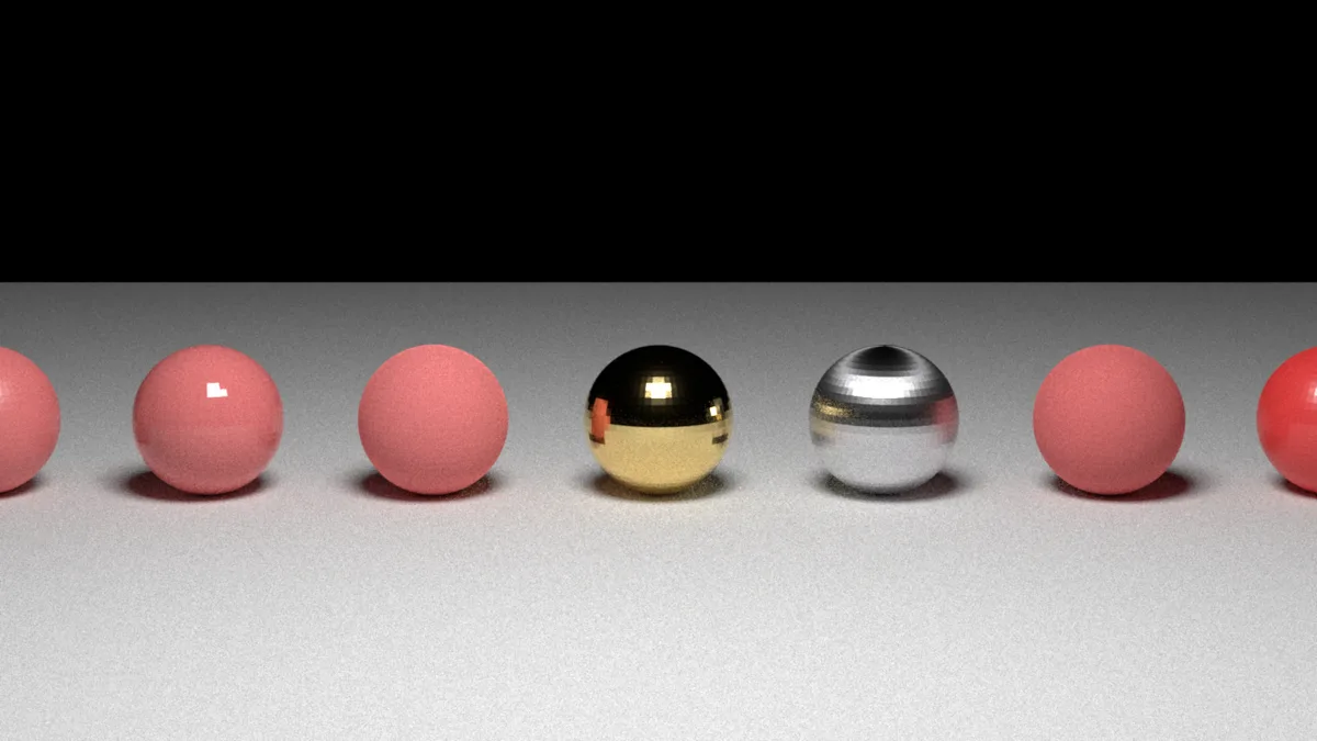
principled BSDF reference render, 256 spp.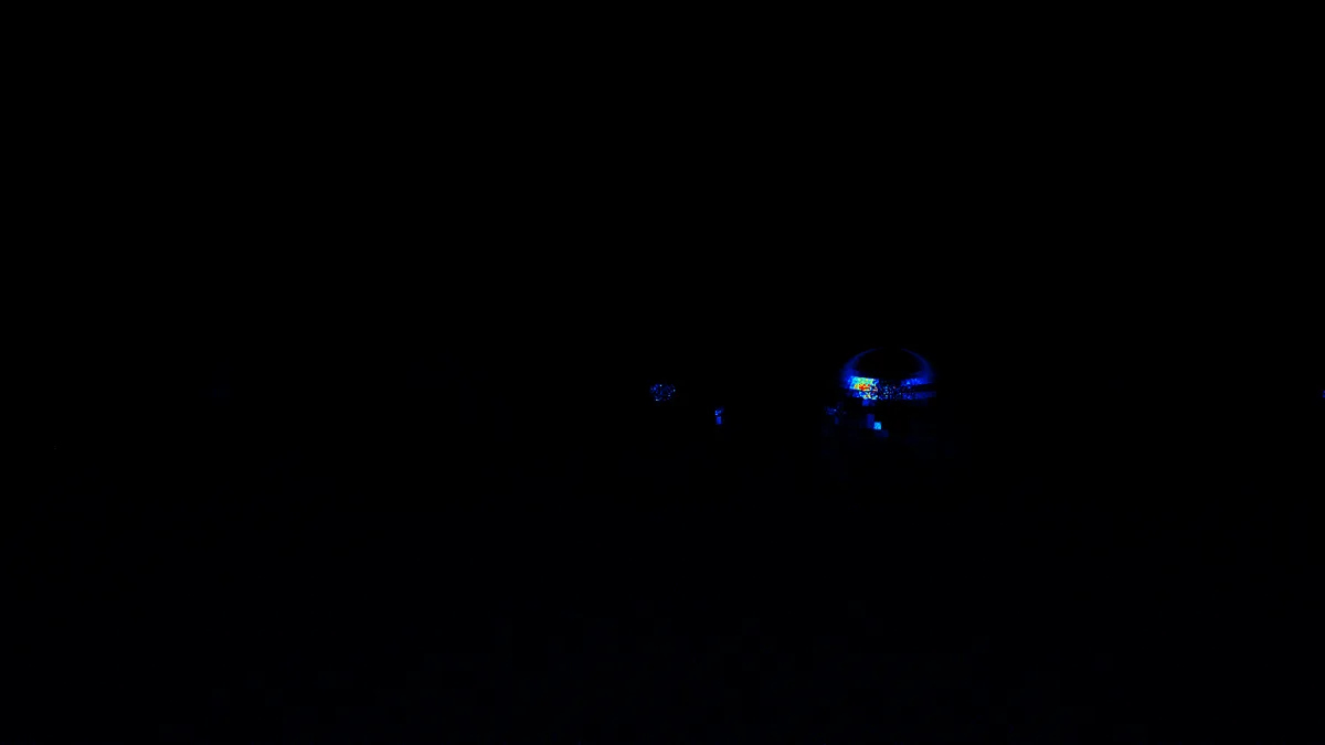
[0, 1] actual MSE scale.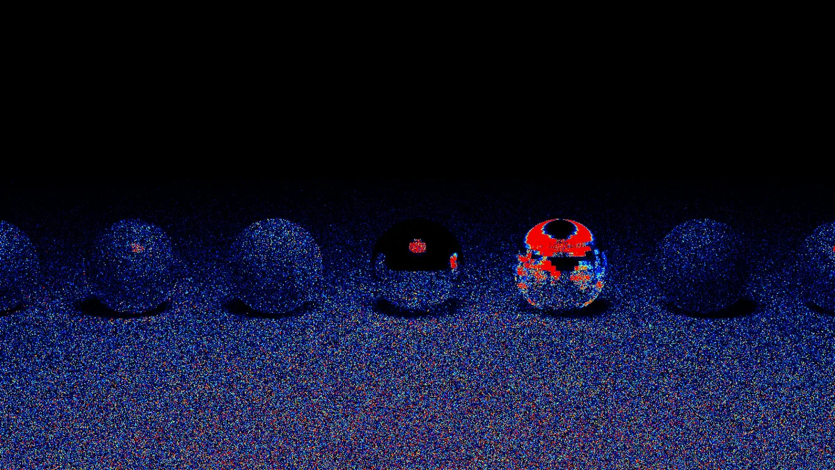
[0, 1e-2] scale.
Source EXRs:
disneyball_showcase_nori_256spp.exr and
disneyball_principled_mitsuba_256spp.exr.
| Metric | Value |
|---|---|
| Global MSE | 1.72238296e-03 |
| Median per-pixel MSE | 4.14021088e-05 |
| 90th percentile per-pixel MSE | 3.67228291e-03 |
| 99th percentile per-pixel MSE | 1.72735788e-02 |
- The comparison grid shows tonemapped PNG previews, while the MSE values are computed directly from the linear EXR images at 1280x720 resolution.
- The per-pixel MSE is computed as mean squared RGB error for each pixel, then averaged over the full image for the global value.
- The largest residual error comes from the anisotropic brushed-metal sphere because the two renderers attach anisotropic axes to different tangent directions.
- The first heatmap uses a
[0, 1]actual MSE range so near-zero differences remain black; the second uses[0, 1e-2]to reveal smaller BRDF, sampling, and filtering differences.
Directional Spot Light
The directional spot emitter provides a position, direction, cone angle, and falloff. It is useful for localized beams through fog, especially in the bus station scene.
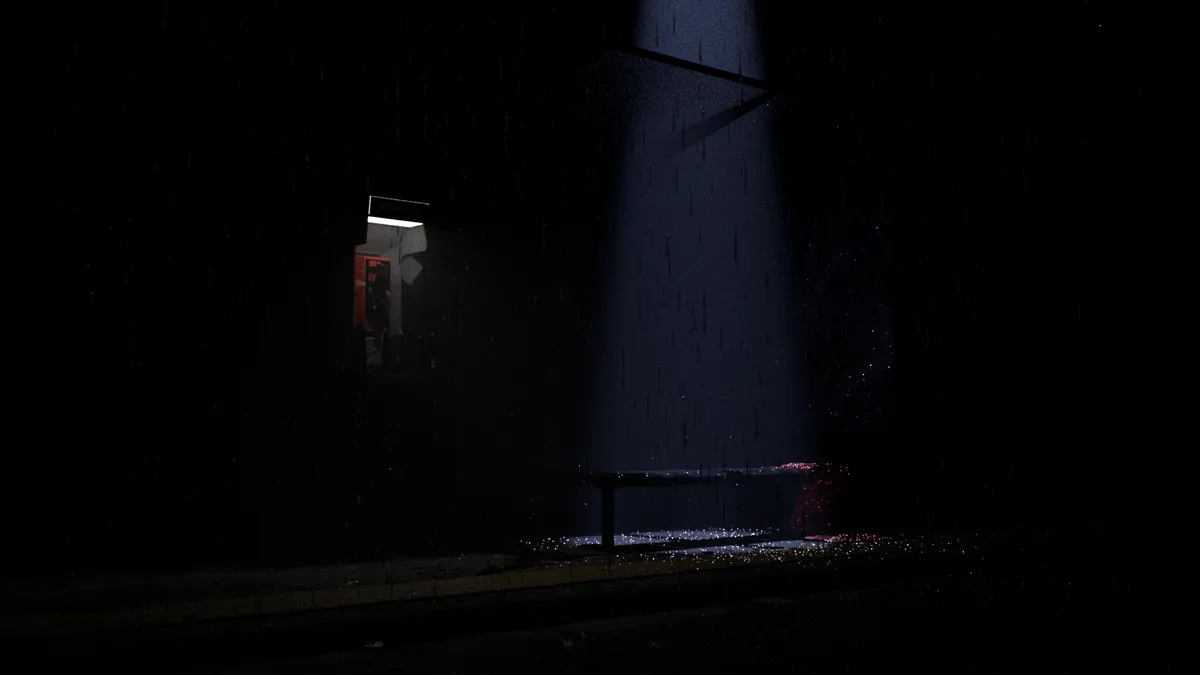
(1500, 2000, 4400).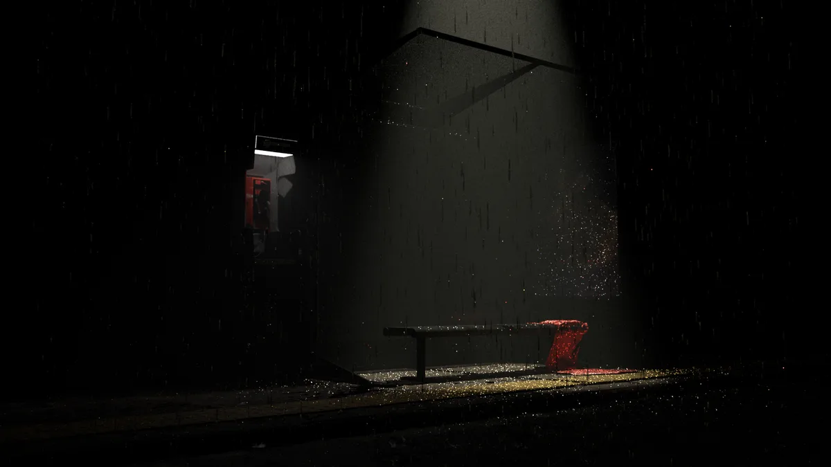
(2000, 2000, 1530).
Rough Dielectric BSDF
The rough dielectric material models glossy transmission and reflection for materials such as frosted or rough glass. It is used in the bus station scene for glass-like surfaces that should not behave like perfectly smooth dielectric.
Validation metrics were computed from the original linear EXR files. Images on this page are compressed web previews; source EXR files are retained locally.
References
- Blender model: Bilibili bus station modeling reference .
- PBRT book: Physically Based Rendering: From Theory to Implementation.
- PBRT GitHub repository: mmp/pbrt-v4.
- Light probe / HDR environment map: Dativ light probes.
- Microcylinder cloth model / reference scene source: A Practical Microcylinder Appearance Model for Cloth Rendering .
- Cloth path tracer reference implementation: MatchaChoco010/path_tracer_cloth.
- Disney BRDF reference: s2012_pbs_disney_brdf_notes_v3.pdf .